Spot modelling with loupiotes

With the example of synthetic data, this tutorial explains how to exploit the ability of the loupiotes Bayesian spot modelling tool.

For more details on the continuous spot model that is used here, see Lanza (2016).

import loupiotes.spots as spots

We start by defining some global properties of the model we are going to use.

inclination, Q = 60, 0
cs, cf0 = 0.67, 0.115
large_dim, reduced_dim = (180, 180), (18,18)
err_data, scale = 500e-6, 0.01
distribution = 'boosted'
timestamps = np.linspace (0, 3*86400, 50)
omega = 8*2.6e-6 #Rotating eight times faster than the Sun

Generating a synthetic model

We are going to work here with synthetic data, the next step is to generate the synthetic map for which we will attempt the spot modelling. This will give a good idea of the possibilities offered by Bayesian spot modelling.

lc_to_fit, err_obs, noise_free, spotmodel_ref = spots.gaussian_noise_lc (timestamps, large_dim=large_dim,
                                                                        reduced_dim=reduced_dim,
                                                                        seed=1389437942, std=err_data, scale=scale,
                                                                        distribution=distribution, boost_std=2.5,
                                                                        return_object=True, inclination=inclination,
                                                                        Q=Q, cs=cs, cf0=cf0, omega=omega)

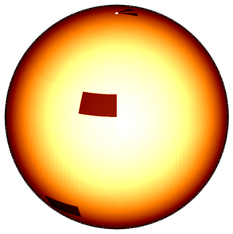
The figure below shows the resolved observed flux at \(t=0\).

fig = spotmodel_ref.plotFluxGrid (figsize=(6,6))

Let’s take a look at the corresponding filling factors \(f_s\) map.

We can also consider the filling factors distribution projected along the longitudinal direction

fig = spotmodel_ref.plotProjectedDistributions (correct_visibility=False)

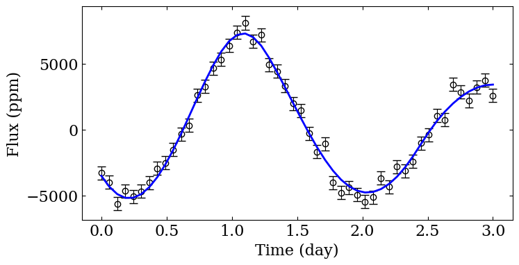
We should also consider the 1D light curve as a function of time.

fig = spotmodel_ref.plotLightCurve (ppm=True, zero_mean=True,
                                    show_errorbars=True, color="blue")

Bayesian model exploration with PyMC

We then proceed to the Bayesian analysis of the generated data, in order to demonstrate which information we can extract from the 1d light curve. This Bayesian procedure is implemented through the PyMC module. A Bayesian sampling can be performed with the Hamiltonian Monte Carlo sampler provided by the module, however given the constraint of the flux grid that are computed by our model, I suggest to do this computation through the use of a GPU. For the sake of this tutorial, we will limit ourselves to the use of a Maximum a-posteriori (MAP) procedure. We start by defining a new SpotModel object.

spotmodel = spots.SpotModel (reduced_dim=reduced_dim, large_dim=large_dim, omega=omega,
                             inclination=inclination, Q=Q, cs=cs, cf0=cf0)

The Bayesian analysis takes place through the explore_distribution function.

result = spotmodel.explore_distribution (timestamps, lc_to_fit, err_data=err_data,
                                         sigma=0.1, use_map=True,
                                         prior_distribution_filling_factors="TruncatedNormal",
                                         )

100.00% [1047/1047 00:18<00:00 logp = 968.43, ||grad|| = 0.072425]

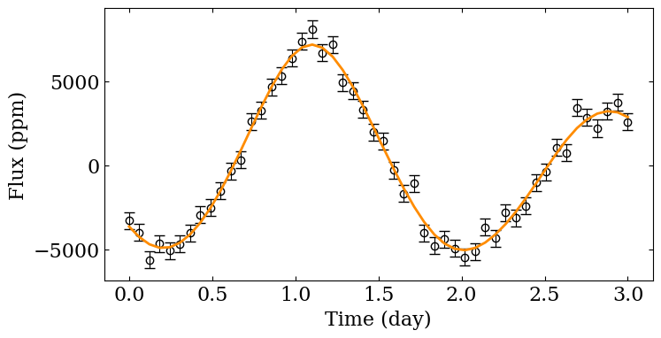
After the sampling, we can compare the light curve target with the one we obtain with the sampling. As visible, there is a very close agreement between both light curve. However, the difficulty of spot modelling does not reside here.

fig = spotmodel.plotLightCurve (ppm=True, zero_mean=True,
                                show_errorbars=True)

The most important is to compare how the sampled filling factor map compared with the synthetic one.

fig = spotmodel_ref.plotProjectedDistributions (correct_visibility=False)
fig = spotmodel.plotProjectedDistributions ()

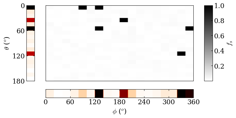
fig = spotmodel.plotFluxGrid (figsize=(6,6))